pacman::p_load(sf, spdep, tmap, tidyverse)Take-home Exercise 2: Regionalisation of Multivariate Water Point Attributes with Non-spatially Constrained and Spatially Constrained Clustering Methods
Overview
Getting Started
Data Import
Import water point data
wp <- read_csv("Take home 2 data/WPdx.csv",show_col_types = FALSE) %>%
  filter(`#clean_country_name` == "Nigeria")
I use
show_col_types = FALSEto avoid warning message.To extract Nigeria data I use
filter()
I saved it into wp_nga.rds. In this way I can delete geo_export data which is too large to git push.
wp_nga<-write_rds(wp,"Take home 2 data/wp_nga.rds")wp_nga <- read_rds("Take home 2 data/wp_nga.rds") Convert wkt data
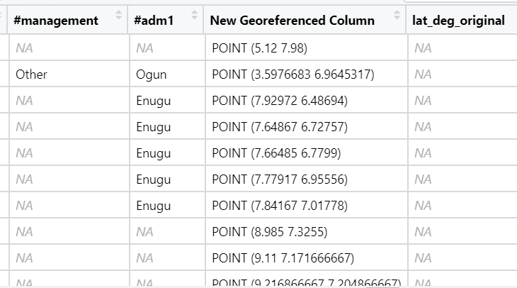
Column ‘New Georaferenced Column’ represent spatial data in a textual format. this kind of text file is popularly known as Well Known Text in short wkt.

Two steps will be used to convert an asptial data file in wkt format into a sf data frame by using sf.
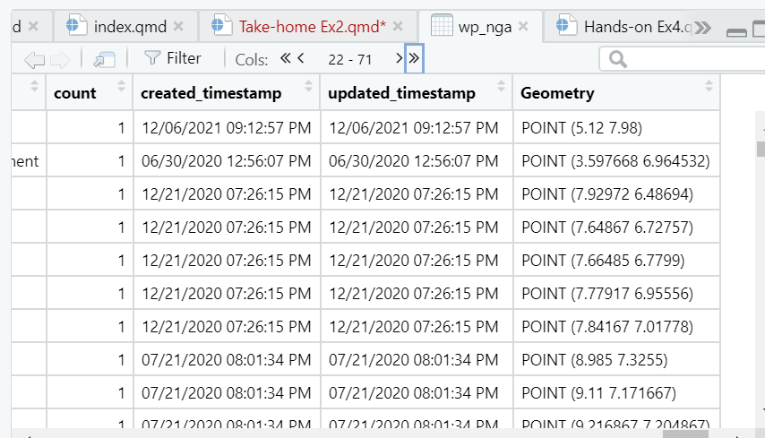
First, st_as_sfc() of sf package is used to derive a new field called Geometry as shown in the code chunk below.
wp_nga$Geometry = st_as_sfc(wp_nga$`New Georeferenced Column`)Now we get the new column called Geometry.

Next, st_sf() will be used to convert the tibble data frame into sf data frame.
wp_sf <- st_sf(wp_nga, crs=4326) When the process completed, a new sf data frame called wp_sf will be created.
Importing Nigeria LGA level boundary data
nga<- st_read(dsn="Take home 2 data",
             layer="geoBoundaries-NGA-ADM2",
             crs=4326)
Reading layer `geoBoundaries-NGA-ADM2' from data source
`D:\Xu-Siyi\ISSS624\Take-home Exercise\Take home 2 data' using driver `ESRI Shapefile'
Simple feature collection with 774 features and 5 fields
Geometry type: MULTIPOLYGON
Dimension: XY
Bounding box: xmin: 2.668534 ymin: 4.273007 xmax: 14.67882 ymax: 13.89442
Geodetic CRS: WGS 84Point in Polygon Overlay
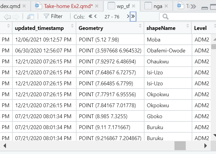
To make sure the data accuracy, we are going to use a geoprocessing function (or commonly know as GIS analysis) called point-in-polygon overlay to transfer the attribute information in nga sf data frame into wp_sf data frame.
wp_sf <- st_join(wp_sf, nga)Now we have column called “shapeName”, which is the LGA name of Nigeria water point.

Data Wrangling
Reference: Ong Zhi Rong Jordan
Checking of duplicated area name
We use duplicate function to retrieve all the shapeName that has duplicates and store it in a list. From the result below, we identified 12 shapeNames that are duplicates.
nga <- (nga[order(nga$shapeName), ])

duplicate_area <- nga$shapeName[ nga$shapeName %in% nga$shapeName[duplicated(nga$shapeName)] ]

duplicate_area
[1] "Bassa" "Bassa" "Ifelodun" "Ifelodun" "Irepodun" "Irepodun"
[7] "Nasarawa" "Nasarawa" "Obi" "Obi" "Surulere" "Surulere"Next, we will leverage on the interactive viewer of tmap to check the location of each area. Through the use of Google, we are able to retrieve the actual name and state of the areas. The table below shows the index and the actual name of the area.
| Index | Actual Area Name |
|---|---|
| 94 | Bassa (Kogi) |
| 95 | Bassa (Plateau) |
| 304 | Ifelodun (Kwara) |
| 305 | Ifelodun (Osun) |
| 355 | Irepodun (Kwara) |
| 356 | Irepodun (Osun) |
| 518 | Nassarawa |
| 546 | Obi (Benue) |
| 547 | Obi(Nasarawa) |
| 693 | Surulere (lagos) |
| 694 | Surulere (Oyo) |
tmap_mode("view")tmap mode set to interactive viewingtm_shape(nga[nga$shapeName %in% duplicate_area,]) +
tm_polygons()Make sure the tmap mode set back to plot
tmap_mode("plot")tmap mode set to plottingWe will now access the individual index of the nga data frame and change the value. Lastly, we use the length() function to ensure there is no more duplicated shapeName.
nga$shapeName[c(94,95,304,305,355,356,519,546,547,693,694)] <- c("Bassa (Kogi)","Bassa (Plateau)",
                                                                               "Ifelodun (Kwara)","Ifelodun (Osun)",
                                                                               "Irepodun (Kwara)","Irepodun (Osun)",
                                                                               "Nassarawa","Obi (Benue)","Obi(Nasarawa)",
                                                                               "Surulere (Lagos)","Surulere (Oyo)")

length((nga$shapeName[ nga$shapeName %in% nga$shapeName[duplicated(nga$shapeName)] ]))
[1] 0Projection of sf dataframe
ngaT <- wp_sf  %>%
  rename ("Country" = "#clean_country_name",
          "clean_adm2" = "#clean_adm2",
          "status" = "#status_clean",
          "lat" = "#lat_deg",
          "long" = "#lon_deg") %>%
  select (clean_adm2,status,lat,long) %>%
  mutate(status = replace_na(status, "Unknown"))

ngaT_sf <- st_as_sf(ngaT, coords = c("long", "lat"),  crs = 4326)
ngaT_sf <- st_transform(ngaT_sf, crs = 26391)
st_crs (nga)Coordinate Reference System:
User input: EPSG:4326
wkt:
GEOGCRS["WGS 84",
ENSEMBLE["World Geodetic System 1984 ensemble",
MEMBER["World Geodetic System 1984 (Transit)"],
MEMBER["World Geodetic System 1984 (G730)"],
MEMBER["World Geodetic System 1984 (G873)"],
MEMBER["World Geodetic System 1984 (G1150)"],
MEMBER["World Geodetic System 1984 (G1674)"],
MEMBER["World Geodetic System 1984 (G1762)"],
MEMBER["World Geodetic System 1984 (G2139)"],
ELLIPSOID["WGS 84",6378137,298.257223563,
LENGTHUNIT["metre",1]],
ENSEMBLEACCURACY[2.0]],
PRIMEM["Greenwich",0,
ANGLEUNIT["degree",0.0174532925199433]],
CS[ellipsoidal,2],
AXIS["geodetic latitude (Lat)",north,
ORDER[1],
ANGLEUNIT["degree",0.0174532925199433]],
AXIS["geodetic longitude (Lon)",east,
ORDER[2],
ANGLEUNIT["degree",0.0174532925199433]],
USAGE[
SCOPE["Horizontal component of 3D system."],
AREA["World."],
BBOX[-90,-180,90,180]],
ID["EPSG",4326]]st_crs (ngaT_sf)Coordinate Reference System:
User input: EPSG:26391
wkt:
PROJCRS["Minna / Nigeria West Belt",
BASEGEOGCRS["Minna",
DATUM["Minna",
ELLIPSOID["Clarke 1880 (RGS)",6378249.145,293.465,
LENGTHUNIT["metre",1]]],
PRIMEM["Greenwich",0,
ANGLEUNIT["degree",0.0174532925199433]],
ID["EPSG",4263]],
CONVERSION["Nigeria West Belt",
METHOD["Transverse Mercator",
ID["EPSG",9807]],
PARAMETER["Latitude of natural origin",4,
ANGLEUNIT["degree",0.0174532925199433],
ID["EPSG",8801]],
PARAMETER["Longitude of natural origin",4.5,
ANGLEUNIT["degree",0.0174532925199433],
ID["EPSG",8802]],
PARAMETER["Scale factor at natural origin",0.99975,
SCALEUNIT["unity",1],
ID["EPSG",8805]],
PARAMETER["False easting",230738.26,
LENGTHUNIT["metre",1],
ID["EPSG",8806]],
PARAMETER["False northing",0,
LENGTHUNIT["metre",1],
ID["EPSG",8807]]],
CS[Cartesian,2],
AXIS["(E)",east,
ORDER[1],
LENGTHUNIT["metre",1]],
AXIS["(N)",north,
ORDER[2],
LENGTHUNIT["metre",1]],
USAGE[
SCOPE["Engineering survey, topographic mapping."],
AREA["Nigeria - onshore west of 6°30'E, onshore and offshore shelf."],
BBOX[3.57,2.69,13.9,6.5]],
ID["EPSG",26391]]Exploratory Data Analysis (EDA)
EDA using statistical graphics
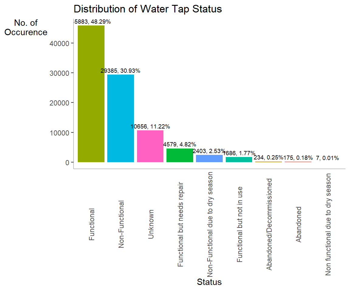
We can plot the distribution of the variables (i.e. Number of households with radio) by using appropriate Exploratory Data Analysis (EDA) as shown in the code chunk below.
Histogram is useful to identify the overall distribution of the data values (i.e. left skew, right skew or normal distribution)
ggplot(data= ngaT_sf,
       aes(x= fct_infreq(status))) +
  geom_bar(aes(fill = status), show.legend = FALSE) +
  geom_text(stat = 'count',
           aes(label= paste0(after_stat(count), ', ',
                             round(after_stat(count)/sum(after_stat(count))*100,
                             2), '%')), vjust= -0.5, size= 2.5) +
  labs(y= 'No. of\nOccurence', x= 'Status',
       title = "Distribution of Water Tap Status") +
  theme(axis.title.y= element_text(angle=0), axis.ticks.x= element_blank(),
        panel.background= element_blank(), axis.line= element_line(color= 'grey'),
        axis.text.x = element_text(angle = 90, vjust = 0.5))